
Monte Carlo Simulation Results
The infinite temperature results: T= K .
For the infinite temperature, consequently the nearest-neighbor coupling J plays no role, and all attempted particle-hole exchange are executed with unit rate. Thus, the vacancies perform a Brownian random walk, regardless of their local environment. Resulting in a rougher interface as time progresses. To illustrate the gradual destruction of the interfaces and the disordering of the bulk, Fig.1 shows the evolution of a typical configuration, in a 60 x 60 system with a single vacancy (represented by a white square in the figure).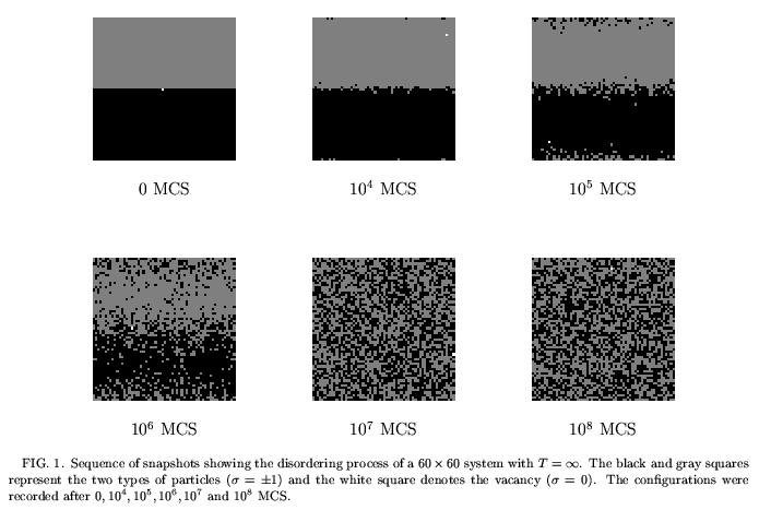
At t=0, the vacancy is located at the interface in the center which begins to break up slowly. Eventually, the second interface also becomes affected. As more particles are transported into regions of opposite color, the system finally becomes completely disordered. For later reference, we note that the last two configurations, at 107 and 108 MCS, are both already fully random. The disordering process is clearly reflected in the number of broken bonds: A(60,t), shown in Fig.2, increases from its minimum of O(L) for the initial configuration at t=0, to O(L2) for the fully equilibrated system at t=107.

One clearly distinguishes three regimes, shown schematically in the inset: the early regime (I), the intermediate or scaling regime (II), and finally the late or saturation regime (III) in which the system has effectively reached the steady state. Tracking the motion of the vacancy, the physical origin of these three regimes is easily identified. For early regime (I), the vacancy is still localized in the vicinity of its starting point, far from the boundaries of the system. After O(L2), however, the vacancy has explored the whole system and is effectively equilibrated. This marks the onset of the intermediate regime (II). The particle distribution is still strongly inhomogeneous and does not equilibrate until the system enters the saturation regime (III). We emphasize that the second and third regimes emerge only in a finite system. In an infinite system, regime (I) persists for all times.
The finite temperature results: Tc < T < K
.When the final temperature of the system is finite, T < K , the full Hamiltonian, Eqn (1) , comes into play when a vacancy attempts to move. In particular, the defects no longer perform a simple random walk, since the jump rates now carry information about the local environment, i.e., the distribution of black and white particles around the originating and receiving site. Thus, a feedback loop between vacancy and background is established, in stark contrast to the case T=K . One might expect that this has significant consequences for profiles and disorder parameter, and that dynamic scaling exponents might be modified. It is immediately obvious that we should distinguish final temperatures above Tc from those below. In the former case, the final steady-state configurations are still homogeneous, even if correlations become more noticeable. In the latter case, however, the equilibrium state itself is phase-separated, so that the only effect of the vacancies is to ``soften'' the initial interfaces. This aspect of vacancy-induced disordering should be particulary interesting in two dimensions, where Ising interfaces are known to be rough[21] . There, the vacancies must mediate both the development of an ``intrinsic interfacial width'' and the emergence of large-scale wanderings of the interface[22]. Certainly, we expect these two phenomena to take place on drastically different time scales, since they are associated with local vs. global disorder.
In this Section, we focus on final temperatures above criticality: Tc< T < K , and a single vacancy, M=1. Starting with a set of typical evolution pictures, we investigate the dynamic scaling properties of the disorder parameter. Since the equations of motion now become highly nonlinear, we have not been able to solve them exactly. Thus, we offer only a few comments in conclusion.

Fig. 3 shows the evolution of a typical configuration, in a 60 x 60 system with a single vacancy at T=1.5Tc. Note that the MC times are the same as in Fig. 1. Again, we observe the gradual, yet eventually complete, destruction of the interfaces. In comparison with Fig. 1, however, two obvious differences emerge: First, the system takes longer time to reach the final steady state. Second, the final configuration shows clear evidence of a finite correlation length. Both features are induced by the interactions. In particular, the disordering process is slowed down since the breaking of bonds is energetically costly. At a more quantitative level, this is documented in Fig. 4 which shows the disorder parameter, for a 60 x 60 system at several temperatures.

One observes that the late crossover time shifts to later times as the temperature decreases. In contrast, the early crossover time appears to be less affected. Also, the saturation value of the disorder parameter decreases. However, being essentially the Ising energy, it remains extensive, with a T-dependent amplitude.
We comment briefly on some analytic results. First, we can conclude that the saturation values, Asat(L), are consistent with exact results for the two-dimensional Ising value. Table 1 shows this comparison for a 60 x 60 system with a single vacancy at several temperatures.

AsatMC is the measured saturation value of the disorder parameter. AsatTH is calculated on the basis of Eqn (2) , where < H> is the exact bulk value for the average energy of the usual Ising model[20]. The effect of the vacancy has been neglected. The agreement is within the statistical errors of our data. The discrepancies are of course largest for the last column, with T closest to Tc.

