Basic descriptive statistics with HISTO
| Index | ||
|---|---|---|
| Visualizing Data | A-Z | Single Raster Analysis Tools Basic descriptive statistics with HISTO |
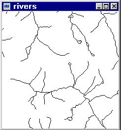
given are a vegetation (raster) and a river (vectors) map.
What we want to find out: do certain plant associations cohere with proximity to rivers?
About the data:
the vegetation has been digitized from a analog copy. The original field data were
superimposed on a 1:25000 map. The whole digital vegetation data exist in form of
a Arc/Info® coverage. The import happened through Arc/Infos UNGENERATE format
and IDRISIs ARCIDRIS module. As the latter produces vectors, a rasterizing process
followed (resolution has been adjusted to 25 m). The river data originated from
1:50000 maps and were treated the same way as the vegetation
information except the rasterizing.
Both data are georeferenced to the same coordinates.
in IDRISI this requires a two-step procedure: (1) INITIAL to create a new empty image for the data to be filled in during rasterize with (2) LINERAS. If desirable IDRISI allows for copying spatial parameters (rows, cols, min x, min y, ...) from an existing image.
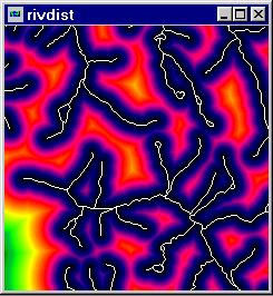
the DISTANCE operator looks for non-zero cellvalues, takes them as a target
and calculates the distances to these cells. The resulting image now holds
euclidian distance values given in reference units. Use SPDIST
where spherical distortions should be avoided. Keep in mind, that DISTANCE calculates
for a 'flat' surface - results do not take into account slopes hence do
not correspond to 'real' distances, especially in steep mountainous areas!
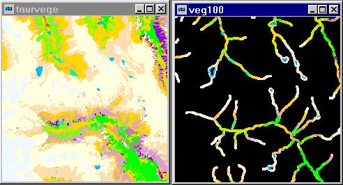
The darker the color the closer we get to a water streamline. For a
better orientation the vector layer rivers has been
overlaid.
Consider the different data resolutions: vegetation on the basis of 1:25000, but rivers digitized from 1:50000 maps. The inspected region is part of the Alps, the rivers should better be delineated as brooks sometimes forming gorges with their own microclimate. For the sake of demonstration we will inspect the image for 100 resp. 300 m distance buffer zones around rivers.
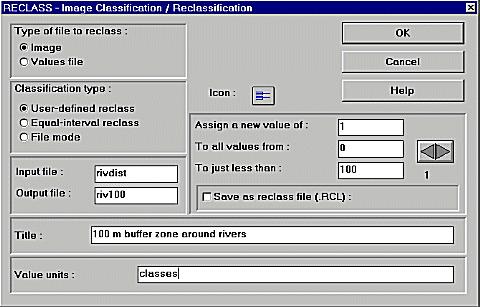
By applying RECLASS to the output image of DISTANCE (rivdist) we extract a 100 m buffer zone around the rivers: distance values between 0 and 100 are set to 1, all others to 0. The output image (here named riv100) contains only 1 and 0, 'yes' and 'no', therefor call it a boolean image
We go on with OVERLAY, a very useful and often employed module when it comes to combine two images through addition, subtraction, multiplication, rationing, etc. The module takes the values of the two input images and proceeds with them according to the Overlay options writing the results to the output image cells:
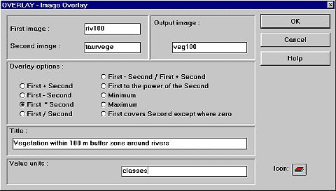
In that we multiply the vegetation with the boolean distance image, only those values (= vegetation classes) survive, that are multiplied with 1 - well, exactly these reside within our desired 100 m buffer zone. Black regions in the illustration below indicate areas outside the 100 m buffer.
We need to stress the module AREA twice - (1) to know the overall
area-size of each vegetation class (taurvege as input image for
AREA) and (2) to get the areas in the buffer
zone (veg100 as input). AREA offers three ways: create an image,
where the cells of each vegetation class receive the summed area of
that class, produce a values file or present the area for the classes
as a table on the screen. In our case it seems appropriate to write out
a values file. Further we must choose area measure units. I took km˛ (number of
cells, m˛, acres, hectares, ... are among the choices).
Repeat the steps starting with RECLASS now with a buffer distance of 300 m.
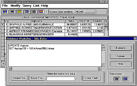
The DATABASE WORKSHOP should be subject of an own exercise, so only
the principal line is sketched here.
We ground the last step on three values files - that one for the areas of
vegetation classes over the whole image, and the others showing the
area sizes of the classes within the 100 resp. 300 m zone. Together with
a values file of the class names a single database can be built up. The
illustration below shows you, how additional database fields can be
calculated from existing ones by standard SQL-statements (here the percentage
of area within buffer zones related to overall area).
Very high percentages mean, that most of the area of that vegetation class resides within a 100 resp. 300 m distance buffer zone. Notice that water does not occupy 100 percent! This fact may well result from the data heterogeneity. Obviously the vegetation map contains a small lake, etc. that is not part of the rivers dataset.
Interpretation and ingenuity of the results in detail may be ceded to experts, but without knowing anything about the vegetation classes, we could make careful assumptions about which associations could be influenced by proximity to waters.
| ID | Vegetation Class Name | Overall area | Area within 100 m zone [km˛] | Area within 300 m zone [km˛] | Percentage 100 m zone | Percentage 300 m zone |
|---|---|---|---|---|---|---|
| 1 | Androsacion alpinae | 56.98687 | 3.693125 | 13.6675 | 6.480659 | 23.98359 |
| 2 | Salicion herbaceae | 6.873125 | 1.083125 | 3.165 | 15.75884 | 46.04892 |
| 3 | Caricion curvulae | 15.14437 | 1.741875 | 5.870625 | 11.5018 | 38.76439 |
| 4 | Seslerio-Semperviretum | 0.44625 | 0 | 0 | 0 | 0 |
| 5 | Aveno-Nardetum | 14.87438 | 1.904375 | 6.308125 | 12.80306 | 42.40934 |
| 6 | Agristio-Trifolio-Deschampsietum cespitosum | 5.370625 | 1.90875 | 3.75 | 35.54056 | 69.82427 |
| 7 | Agrostio-Trifolio-Deschampsion | 2.3525 | 0.853125 | 1.9525 | 36.26461 | 82.99681 |
| 8 | Polygono-Trisetion | 0.51 | 0.324375 | 0.51 | 63.60294 | 100 |
| 9 | Dactylo-Poion | 0.023125 | 0.005625 | 0.023125 | 24.32433 | 100 |
| 10 | Brachypodio-Koelerietum | 0.021875 | 0 | 0.0075 | 0 | 34.28571 |
| 11 | Loiseleurietum | 3.27 | 0.49625 | 1.56875 | 15.17584 | 47.97401 |
| 12 | Rhododendretum ferruginei | 5.620625 | 0.94 | 2.718125 | 16.72412 | 48.35984 |
| 13 | Erico-Rhododendretum hirsuti | 0.00375 | 0 | 0 | 0 | 0 |
| 14 | Junipero-Callunetum | 0.721875 | 0.055 | 0.25 | 7.619048 | 34.63203 |
| 15 | Pinetum mugli | 1.406875 | 0.114375 | 0.39125 | 8.129721 | 27.80986 |
| 16 | Alnetum viridis | 5.616875 | 1.17625 | 3.28125 | 20.94136 | 58.41771 |
| 17 | Cembretum | 0.449375 | 0.026875 | 0.214375 | 5.980528 | 47.70515 |
| 18 | Larici-Cembretum | 1.659375 | 0.1075 | 0.585625 | 6.478343 | 35.2919 |
| 19 | Vaccinio-Rhododendro-Laricetum | 0.198125 | 0.020625 | 0.0625 | 10.4101 | 31.54574 |
| 20 | Larici-Piceetum | 4.884375 | 1.44125 | 3.6775 | 29.50736 | 75.29111 |
| 21 | Piceetum subalpinum | 0.00625 | 0 | 0.00625 | 0 | 100 |
| 22 | Luzulo-Piceetum | 2.3575 | 0.829375 | 1.846875 | 35.18027 | 78.3404 |
| 23 | Alnetum incanae | 0.160625 | 0.1 | 0.160625 | 62.25681 | 100 |
| 24 | Salicetum eleagni | 0.053125 | 0.025 | 0.053125 | 47.05882 | 100 |
| 25 | Adenostyletalia | 1.048125 | 0.1375 | 0.603125 | 13.11866 | 57.54323 |
| 26 | Dryopteridetum | 0.323125 | 0.071875 | 0.254375 | 22.24371 | 78.7234 |
| 27 | Caricion fuscae | 0.475625 | 0.28125 | 0.444375 | 59.13272 | 93.4297 |
| 28 | very moist soils and fountain areas | 0.301875 | 0.194375 | 0.301875 | 64.38924 | 100 |
| 29 | Glaciers | 11.6075 | 0.136875 | 0.723125 | 1.179194 | 6.229808 |
| 30 | Waters | 0.8275 | 0.6275 | 0.78625 | 75.83082 | 95.01511 |
| 31 | Other regions (scree flora or cultivated areas) | 0.404375 | 0.054375 | 0.08125 | 13.44668 | 20.09274 |
| Index | ||
|---|---|---|
| Visualizing Data | A-Z | Single Raster Analysis Tools Basic descriptive statistics with HISTO |