Visualizational aspects
Classification - unsupervised
| Index | ||
|---|---|---|
| Image Processing IV Visualizational aspects |
A-Z | Image Processing V Classification - unsupervised |
The techniques brought up here fit in more functional categories, so do not strictly rely upon this outline. More thorough discussions of the following topics would require lots more space, so I strongly recommend reading (geo)statistical textbooks (also check the recently published sample exercise from the Remote Sensing Core Curriculum about Principal Components Analysis).
Data reduction - PCA (Principal Components Analysis)Link back to the previous page and take a look at the 7 spectral bands from the Landsat TM data. You may notice more or less strong correspondence in the data - these are redundancies, 'digital ballast' not always necessary to carry along with the data. With the statistical method of principal components analysis we 'extract the essentials' by producing so-called 'principal component images' and statistical information output in IDRISI:
| Table: PCA tabular output in IDRISI 7 spectral bands were feed into the PCA-function to produce 7 components | |||||||||
|---|---|---|---|---|---|---|---|---|---|
| VAR/COVAR | taurtm1 | taurtm2 | taurtm3 | taurtm4 | taurtm5 | taurtm6 | taurtm7 |
| |
| taurtm1 | 3087.33 | 2070.67 | 2530.54 | 974.94 | -517.63 | -449.01 | -34.25 | ||
| taurtm2 | 2070.67 | 1546.11 | 1842.13 | 844.92 | -359.73 | -300.25 | -54.99 | ||
| taurtm3 | 2530.54 | 1842.13 | 2218.84 | 960.56 | -411.23 | -362.97 | -38.62 | ||
| taurtm4 | 974.94 | 844.92 | 960.56 | 1063.28 | 106.61 | -16.30 | -22.00 | ||
| taurtm5 | -517.63 | -359.73 | -411.23 | 106.61 | 1021.40 | 288.10 | 482.89 | ||
| taurtm6 | -449.01 | -300.25 | -362.97 | -16.30 | 288.10 | 157.74 | 97.38 | ||
| taurtm7 | -34.25 | -54.99 | -38.62 | -22.00 | 482.89 | 97.38 | 290.16 | ||
| COR-MATRX | taurtm1 | taurtm2 | taurtm3 | taurtm4 | taurtm5 | taurtm6 | taurtm7 |
| |
| taurtm1 | 1.000000 | 0.947761 | 0.966847 | 0.538101 | -0.291492 | -0.643424 | -0.036191 | ||
| taurtm2 | 0.947761 | 1.000000 | 0.994571 | 0.658977 | -0.286261 | -0.607986 | -0.082100 | ||
| taurtm3 | 0.966847 | 0.994571 | 1.000000 | 0.625371 | -0.273162 | -0.613545 | -0.048126 | ||
| taurtm4 | 0.538101 | 0.658977 | 0.625371 | 1.000000 | 0.102303 | -0.039810 | -0.039612 | ||
| taurtm5 | -0.291492 | -0.286261 | -0.273162 | 0.102303 | 1.000000 | 0.717772 | 0.887027 | ||
| taurtm6 | -0.643424 | -0.607986 | -0.613545 | -0.039810 | 0.717772 | 1.000000 | 0.455205 | ||
| taurtm7 | -0.036191 | -0.082100 | -0.048126 | -0.039612 | 0.887027 | 0.455205 | 1.000000 | ||
| COMPONENT | C1 | C2 | C3 | C4 | C5 | C6 | C7 |
| |
| %var. | 77.51 | 14.42 | 6.45 | 1.08 | 0.37 | 0.10 | 0.06 | ||
| eigenval. | 7274.64 | 1353.37 | 605.34 | 101.62 | 34.36 | 9.61 | 5.92 | ||
| eigvec.1 | 0.637395 | -0.024205 | -0.332783 | -0.664908 | 0.078396 | -0.128519 | -0.132783 |
| |
| eigvec.2 | 0.453689 | 0.032000 | 0.011831 | 0.568448 | 0.035183 | 0.001237 | -0.684566 | ||
| eigvec.3 | 0.551395 | 0.026079 | -0.050350 | 0.419740 | 0.048126 | -0.022627 | 0.716756 | ||
| eigvec.4 | 0.250048 | 0.409488 | 0.816091 | -0.233731 | -0.101826 | 0.196958 | 0.000000 | ||
| eigvec.5 | -0.111267 | 0.798522 | -0.256041 | 0.062861 | -0.203832 | -0.488801 | 0.000000 | ||
| eigvec.6 | -0.092584 | 0.210568 | 0.060913 | 0.000970 | 0.968702 | -0.070669 | 0.000000 | ||
| eigvec.7 | -0.019534 | 0.384777 | -0.388984 | 0.000205 | 0.000000 | 0.836813 | 0.000000 | ||
| LOADING | C1 | C2 | C3 | C4 | C5 | C6 | C7 |
| |
| taurtm1 | 0.978414 | -0.016026 | -0.147356 | -0.120630 | 0.008270 | -0.007172 | -0.005814 | ||
| taurtm2 | 0.984110 | 0.029939 | 0.007403 | 0.145732 | 0.005245 | 0.000098 | -0.042358 | ||
| taurtm3 | 0.998401 | 0.020367 | -0.026299 | 0.089826 | 0.005989 | -0.001489 | 0.037021 | ||
| taurtm4 | 0.654042 | 0.461983 | 0.615764 | -0.072257 | -0.018305 | 0.018729 | 0.000000 | ||
| taurtm5 | -0.296944 | 0.919171 | -0.197110 | 0.019828 | -0.037385 | -0.047423 | 0.000000 | ||
| taurtm6 | -0.628746 | 0.616786 | 0.119328 | 0.000778 | 0.452112 | -0.017447 | 0.000000 | ||
| taurtm7 | -0.097810 | 0.830999 | -0.561843 | 0.000121 | 0.000000 | 0.152325 | 0.000000 | ||
If you are not familiar with techies like 'eigenvalue', 'eigenvector', ... I recommend again diving deeper with statistical textbooks. To give you an expression of how that component images look like - find here 7 images from a subscene of the Hohe Tauern region (around the Matreier Tauernhaus):
Component 1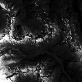 |
Component 2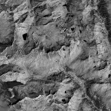 |
Component 3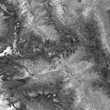 |
Component 4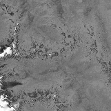 |
Component 5 |
Component 6 |
Component 7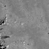 |
||
Such images might be simply used for enhancement, data reduction or even later on in the classification process (be careful in using them in the latter). Helpful not only for interpreting the results of the PCA are additional XY-scatterplots of one band versus another. In the IDRISI for DOS version you could create simple scatterplots with the routine SCATTER. The following scatterplot matrix has been prepared with the help of SPSS 7.0:
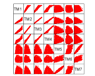 e.g., 'TM 1' means thematic mapper band 1;
compare these plots against the correlation matrix part of the IDRISI output. Clearly visible are strong positive linear correlations between bands 2 + 3, 2 + 4, 3 + 4.
| Index | ||
|---|---|---|
| Image Processing IV Visualizational aspects |
A-Z | Image Processing V Classification - unsupervised |