Index
Single Raster Analysis Tools V QUADRAT, CENTER - Point Pattern Analysis	A-Z	Single Raster Analysis Tools VII AUTOCORR - Spatial Autocorrelation

Single Raster Analysis Tools VI

• Interpolation methods in IDRISI - a coarse overview
  This chapter would honestly require to go far back, as interpolation is a rather delicate field in GIS. The interpolation methods in IDRISI and their depth of implementation are confined to the very basics at the moment. Enough to demonstrate principles though.

  Now what is interpolation all about? These are geostatistical ways to estimate information for locations without such, by founding on known surrounding values. Easy to understand the concept, if you imagine height points for some area which you gathered in the field using modern GPS (Global Positioning System). By interpolating between the known height spots you try to build a continuous surface, a DEM. Or you already have some analog maps showing the elevation isolines - again you could rely on known values (in that case: the height lines) to interpolate the unknown elevation between them.

  Getting some results is quite easy - indeed a matter of doing a few clicks! Our computer works hard and the outputs often look very reasonable at the first glance.
  -- But: what did we really get? how reliable are the values compared to reality??
  What may sound as a simple task has more but one trap! To achieve good results one has to be very careful in choosing the 'right' interpolation method and in interpreting the outputs. Those of you interested in underlying algorithms, read David F. WATSON: 'Contouring: A Guide to the Analysis and Display of Spatial Data' (Pergamon Press, Oxford 1992) or Edward H. ISAAKS & R. Mohan SRIVASTAVA 'Applied Geostatistics' (Oxford Univ. Press, Oxford 1989) among several others.

  • TREND
    First, TREND isn't a method to calculate unknown values for specific locations - it is what its name states: it shows larger scale trends, patterns within our data. Statistical basis is the solving of polynomial equations, where IDRISI gives you the choice of 3 orders:
    
    • linear: z(x,y) = b₀ + b₁x + b₂y
    • quadratic: z(x,y) = b₀ + b₁x + b₂y + b₃x² + b₄xy + b₅y²
    • cubic: z(x,y) = b₀ + b₁x + b₂y + b₃x² + b₄xy + b₅y² + b₆x³ + b₇x²y + b₈xy² + b₉y³
    x, y are the coordinates, z is the attribute value (must be of interval scale at least).

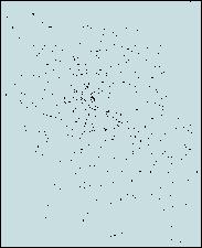
    To give an example (very simplified): following you see a map of 453 point locations in the City of Salzburg with the attribute: number of different lichen species at this point (lichens are those strange plant organisms made up from some kind of symbiotic living-together fungus with algae :-); rather valuable bioindicators!). For the ease of demonstration we make the assumption, that habitat quality is positively correlated with the number of different lichen species per location (data from collection in 1982, ZIEGELBERGER & TÜRK, Salzburg Univ., Dept. of Plantphysiology)

    

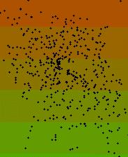
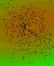
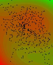
    Now let us compute the trend-images:
    linear, quadratic, cubic
    (red = less species / green = more species per sample location)

    

    IDRISI finishes the TREND-calculation by presenting you some statistics (Goodness of fit, F ratio, degrees of freedom, ...) that can be compared between different trend orders to proof for the significance. Goodness of fit tells about the 'amount of variation explained' through the 'fit'. It is computed by examining the residuals:
    z_i ... observed values
    ... model-predicted values
    ... mean of observed values
    
    

    The above images show a very general pattern of the lichen distribution. Note the increasing complexity from the simple linear (left) to the cubic (right) surface. The quadratic (middle) and the cubic trend images seem to indicate a center of lower species counts in the northern half of the City of Salzburg, which very coarse reflects the situation in reality. But if you focus on the lower left corner of the right result you will notice a zone of apparently lower species counts. It is evident, that there are very few measure points arround, so extrapolation will occur, which makes this results very doubtful.

  • INTERCON
    With the help of this module you may derive DEMs from contour lines. INTERCON requires the contours to be an image, so the whole procedure starts with (1) converting the vector sources into a raster (see 1^st Example, topic 1 for the rasterizing steps). Pay attention to the initial value given to the empty image in INITIAL. It should not be any height value (e.g., do not use 1, if there will be heights of 1 in your DEM). (2) The INTERCON routine asks you for the heights of the four edges. You will maybe have to estimate them. IDRISI then constructs several profiles: a boundary profile from the four edges and any height contour that intersects with the border, a horizontal profile across the rows, a vertical one across the columns and two diagonal (upper left to lower right, upper right to lower left). While making the profile, the program records the slopes for the locations between known height contours and finally assigns the height computed from the maximum slope profile. (3) To get rid of minor inconsistencies, apply a mean filter to the INTERCON-result (at least once) to smooth the DEM.

  • INTERPOL
    Whereas TREND performs a global interpolation, INTERPOL does a local one. It offers two methods: Inverse Distance Weighting (IDW) and Potential Surface Calculation. The latter is being refined currently, so I will not make remarks on it.

    IDW: look at the formula and the line chart below - we calculate estimates of unknown values dependent on neighbouring known values. The distance acts as weight and its exponent allows further adjustment of that weight: the higher the distance exponent, the higher the influence of the nearest known feature value:

    ... interpolated z-value
    d ... distance from known point i
    z ... z-value of known point i
    p ... distance weight exponent
    n ... number of points to be included in search (in IDRISI: six-on-average or all)
    i ... number of known value points to be taken into account
    
    

    These are just six random choosen sample distance values. They indicate the distance from the point to be estimated to the next six known value points in ascending order (the weights have been standardized). Note how the weights of the different distances diverge with higher exponents.
    

    The dialog box of INTERPOL:

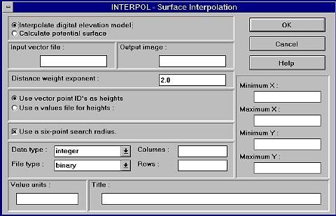    The decision, which parameter combination to use isn't always easy. Look the results over very critical. Here's an excerpt from the IDRISI for WINDOWS Help on the INTERPOL function:

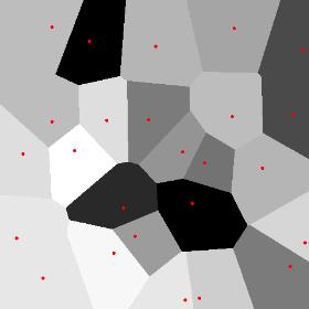
    Do not assume that because a computer has done the interpolation that it has any strong claim to accuracy. There are many interpolation procedures, appropriate for different surface characteristics, and this is only one. The weighted-average technique used produces quite smooth surfaces with maxima and minima occurring at the locations of control points. As one moves away from these control points, the surface will tend towards the local average height, where local is determined by the search radius.
    

  • THIESSEN
    Another way in the point-to-area methods is provided through THIESSEN. This function requires vector points or images with single non-zero cells as points to perform what is generally known as Voronoi Tesselation - the generation of Thiessen Polygons: each point, resp. cell in the output image is allocated to the nearest known point.

    See an example:

    

	Index
Single Raster Analysis Tools V QUADRAT, CENTER - Point Pattern Analysis	A-Z	Single Raster Analysis Tools VII AUTOCORR - Spatial Autocorrelation

last modified: | Comments to Eric J. LORUP