Index
Single Raster Analysis Tools VI Interpolation methods in IDRISI	A-Z	Single Raster Analysis Tools VIII FUZZY

Single Raster Analysis Tools VII

• AUTOCORR - Some notes on spatial autocorrelation
  Autocorrelation is better known from the fields of time series analysis. It denotes a method to study similarity/dissimilarity of the same variables between corresponding intervals. Those intervals (lags) may be of temporal or spatial nature.

  Who whispered: 'Boy, another formula! Another index number describing whatsoever! Who cares?!'.
  That's exactly the point: everyone should care, who uses statistics which are based on an assumption of independence! A lot of spatial related test methods may be rather doubtful, as autocorrelation could lead to heavy biased results!

  To give an practical example: when fitting models to spatial data (regression models, trend surfaces), the residuals must not be spatially autocorrelated. Autocorrelation would indicate 'leakiness' of our model, some minor patterns or variations it did not catch. We then should work it over again.

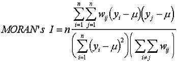
  IDRISI's AUTOCORR function is prepared to compute a spatial autocorrelation index known as MORAN's I:

  	n ........	number of values to be taken into account (cells in our case)
  	w ........	spatial weights: 1 in the directions up/down/left/right, 0.70711 (square root of 2) as weight for the diagonal neighbouring cells
  	yi/j ......	value at location i resp. j (simply number the cells by sequence)
  	µ ........	mean of values y

  This algorithm is implemented in IDRISI such that we are faced with two choices:

  • Rook's case - think of the chess game and how you're allowed to move the rook basically! In the same manner we look at each cells upper, lower, left and right adjacent cells to calculate the index
  • King's case - additionally to Rook's case we add the diagonal neighbours too

  To be complete: IDRISI also allows for masking the image to limit our area of interest. All cells, where the mask-image shows non-zero values are included in the calculation (provided that both images have matching spatial dimensions).

  There is no specific rule about the choice of the weights in general (s. BAILEY & GATRELL 1995^*). Dealing with regular datasets (as is the case in an image without a mask) makes weighting much more feasible than with irregular spaced observations.

  AUTOCORR computes MORAN's I for the first lag only, that means it scans through the whole image and looks at each cell and its immediate neighbours. Exactly this possible dependency on spatial neighbourhood is what we are interested in. So we would like to compute not only for the 1^st lag but also for the 2^nd, 3^rd and so on. We have to be a bit tricky: to get MORAN's I for the 2^nd lag, we first remove every 2^nd pixel from our image by using CONTRACT and then running AUTOCORR. Attention: this trick does not correctly compute the subsequent lags, as CONTRACT thins or aggregates cells, what means loss resp. bias in original data!

  MORAN's I in most cases range between -1 and +1, where +1 means absolute and 0 none spatial autocorrelation. A negative index could indicate some kind of regular pattern. Additionally AUTOCORR outputs several measurements to test for significance of MORAN's I. If no autocorrelation is present, the expected value of I is -1/(n-1). The outputs below are simply too small numbers for the display.

  The datasets used to show the IDRISI output are choosen only because of their nearly perfect autocorrelation/non-autocorrelation.

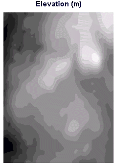
  Here are the results for a sample DEM image from the Harvard Forest dataset:

  Image :ele-m Case :Rook's Case Number of cells included = 67710 Mean of cells included = 351.9728 Standard Deviation (sigma) of cell values = 0.0996 The 3rd number above is in fact the 'Standard Error of Mean' not the Std. dev. Spatial Autocorrelation (Moran's I) = 0.9955 Expected value of I if not autocorrelated = -0.0000 Variance of I (normality assumption) = 0.0000 Variance of I (randomization assumption) = 0.0000 z test stat (normality assumption) = 365.6350 z test stat (randomization assumption) = 365.6348

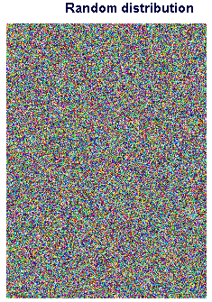
  To make the difference clear, I have computed MORAN's I for an image created by RANDOM, another IDRISI tool. Distribution of values in that image is random:

  Image :random Case :Rook's Case Number of cells included = 67710 Mean of cells included = 50.0225 Standard Deviation (sigma) of cell values = 0.1121 The 3rd number above is in fact the 'Standard Error of Mean' not the Std. dev. Spatial Autocorrelation (Moran's I) = -0.0029 Expected value of I if not autocorrelated = -0.0000 Variance of I (normality assumption) = 0.0000 Variance of I (randomization assumption) = 0.0000 z test stat (normality assumption) = -1.0472 z test stat (randomization assumption) = -1.0472

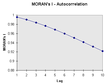
  The following diagram shows the coherence between distance (lag) and MORAN's I (MORAN-Correlogram). Values have been taken from the Harvard Forest DEM and MORAN's I computed from subsequently CONTRACTed DEMs:

  

^* Trevor C. BAILEY & Anthony C. GATRELL, 1995: Interactive Spatial Data Analysis. Longman, Essex.

	Index
Single Raster Analysis Tools VI Interpolation methods in IDRISI	A-Z	Single Raster Analysis Tools VIII FUZZY

last modified: | Comments to Eric J. LORUP